|
XtalView D.E. McRee Molecular Biology, The Scripps Research Institute, La Jolla, CA 92117, USA dem@scripps.edu http://www.scripps.edu/pub/dem-web/lab.html
M. Israel Molecular Biology, The Scripps Research Institute, La Jolla, CA 92117, USA misrael@scripps.edu http://www.scripps.edu/pub/dem-web/misrael.html
|
Abstract
XtalView is a windows-based, interactive crystallographic package developed at The Scripps Research Institute and distributed by CCMS. XtalView has as its main goals portability across many operating systems, extensibility and ease of use. In addition to discussing XtalView in general, I will provide an update on XtalView progress over the last year. A semi-automated fitting module has been added to Xfit that can help trace a protein main chain quickly. We have also added a spline description of maps that allows more accurate interpolation of maps in order to improve contouring, real-space refinement and NCS averaging. A tutorial covering these features and solving Patterson maps with XtalView will be presented.
1 Introduction
XtalView is a crystallographic software package that is designed to be interactive and visual1. The programs run on systems with UNIX and X11. The programs are written at The Scripps Research Institute and distributed by the Computational Center for Macromolecular Structures (CCMS, http://www.sdsc.edu/CCMS/, academic only) at the San Diego Computer Center, and commercially by MSI (Molecular Simulations, Inc., http://www.msi.com). The main uses of XtalView are heavy atom phasing, map contouring, map fitting and molecular modeling.
In order to achieve portability, we decided to use XView (hence the name), which is public domain and available for a large range of platforms. XView also had the advantage that it had one of the few graphical editors available in 1991, when the package was started. Over time the choice of XView has been both a benefit and a liability. I only put this explanation here to dampen somewhat the religious infighting that results when discussing GUIs.
XtalView is organized around the concept of a crystal and a project. A crystal is a file containing unit cell, spacegroup and non-crystallographic symmetry information about a crystal-type. Commonly there will be many datasets that share this information. To supply this information to the programs, the crystal name is passed. A project is a directory and default crystal. Typically a project uses one crystal but sometimes several may be used.
XtalView also creates history files with the extension .hist to keep track of the extensive data path. These files are all compact to take up minimal disk space and should not be deleted (until the paper is published). They allow backtracking to find out where things went wrong and also allow reproducing large files that may have been deleted to save disk space.
The user interface to XtalView has as its aim to provide a visual interface to what was traditionally a card-punch and line-printer oriented computing field - namely macromolecular computing. The user should be able to find program options by browsing the screen and see output in a graphical manner when appropriate. The user may not know what a field does by simple inspection but it does give a starting point for using help. One of the most glaring flaws in XtalView is the lack of context-sensitive help. Unfortunately this proved to be very clumsy to implement with XView across multiple platforms. There is, however, online help in man pages, in a printed manual, and on the World Wide Web at CCMS.
In the past year we have added semi-automated fitting to the XtalView module, Xfit, which makes chain tracing and initial model building much faster and more accurate. Several proteins have been fit at TSRI with these features, and it has resulted in a rapid initial model with correct backbone stereochemistry. We have also added a spline-based map description, in collaboration with Erik Nelson and Lynn Ten Eyck at the University of California at San Diego, which greatly improves the accuracy of the map between grid points.
Another major feature to be implemented is a density modification package that will use solvent flattening, histogram matching and non-crystallographic symmetry averaging to improve phases. The package is currently running as a shell-file implementation. It will be implemented as part of Xfit in a manner that will give the user interactive control over the control parameters. It should also be fairly fast as it will be done completely in memory.
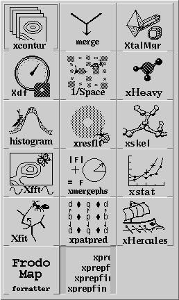
1.0 XtalView Programs
Table 1. XtalView applications
|
Application |
Description |
|
xcontur |
Density map contouring and printing |
|
xdf |
Disk free meter |
|
xedh |
Electron density histograms |
|
xfft |
Fast-Fourier-Transform of electron density and Patterson maps |
|
xfit |
Fitting and model building; Display of electron density |
|
xheavy |
Refinement of MIR data and calculation of phases |
|
xmerge |
Merge and Scale datasets |
|
xmergephs |
Phase mutant data with native phases; cross Fouriers; Bijvoet difference Fourier |
|
xpatpred |
Predict Patterson peaks from trial solutions - display solution with xcontur |
|
xprepfin |
Import/Export data to XtalView, reduce indices, fix various possible problems |
|
xresflt |
Resolution filter |
|
xrspace |
Reciprocal Space viewer to check data completeness, symmetries, etc. |
|
xtalmgr |
Top level of XtalView. Manages database, files, and projects. Launches applications |
|
xhercules |
Automated Patterson map solving |
|
stfact |
Calculate structure factors from PDB files |
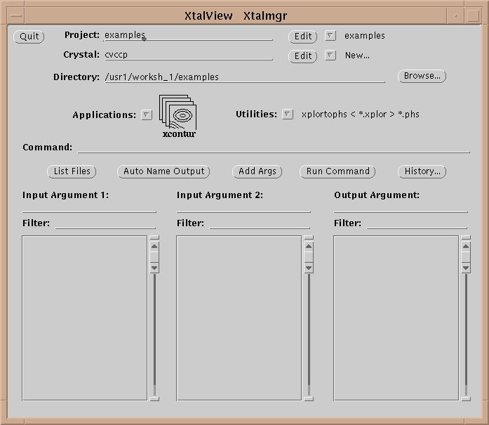
Table 1 lists the XtalView programs. An XtalView session starts with xtalmgr, which is used to launch the other applications with the appropriate files:
The first operation is to set a project by either selecting one with the menu button or editing a new one if it does not exist. If the crystal does not exist yet, edit it by selecting the Edit button (![]() ):
):
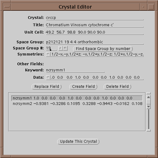
In this window one can edit the parameters of a crystal. In particular all 240 space groups are known and can be found by entering the symbol on the Space Group line and hitting return or by setting the space group number field and selecting Find Space Group by Number. Each crystal is given a unique keyword in the Crystal field. When done updating the information, select Update This Crystal to store the information in the database.
The directory in xtalmgr is usually set by setting the project. However, one can also manually set the directory by typing it in or using the Browse… button. The Browse window also allows deleting files.
Having set the crystal and directory, either by choosing a project or by entering them specifically, an application needs to be chosen. Use the application menu button ![]() to bring up a list of applications:
to bring up a list of applications:
Drag the mouse over, and select one of the applications by choosing its icon. This will cause xtalmgr to list the files that can be used by that application and to start building a command line. To finish the command line you need to choose one or two input files from the lists by clicking on them. If you need an output file, you can either enter a name or use the Auto Name Output button to make up a name from the input file[s]. The filenames are then added with the Add Args button, and the command launched with Run Command.
The following gives short descriptions of common applications of XtalView to give a flavor of what the programs can do. The best way to learn the programs is to plunge in and start playing. Be sure to explore all the menus and options.
1.1 Preparing Data
The main file format used in XtalView is the .fin file. .fin files have the following format:
h k l F1 sigma(F1) F2 sigma(F2)
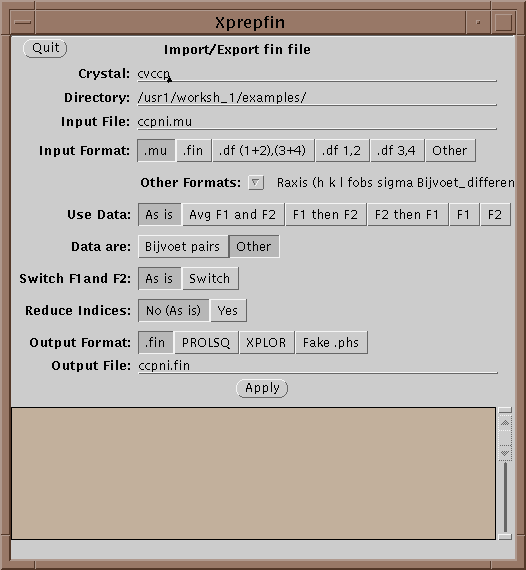
The files are free-format, where hkl are integers and the rest are reals. If either F1 or F2 is missing then it should be entered as 0.0 with the sigma greater than or equal to 9999.0. Xprepfin contains a number of routines for converting popular formats. You can also add a new one by editing and following the instructions in $XTALVIEWHOME/data/OtherFormats. To do this a filter program is needed that takes as standard input (unit 5 in FORTRAN) the format to be converted and outputs to standard out (unit 6 in FORTRAN) .fin format.
In a typical .fin file F1 and F2 represent the amplitudes of Bijvoet pairs, F+ and F-. The other common format is to have two merged datasets such as native data and heavy atom data: Fnat and Fheavy, or Fwildtype and Fmutant. The main difference is in how to handle centric reflections. With Bijvoet pair data, centrics do not have a Bijvoet pair, and this is indicated by having F- set to 0.0 and its sigma set to 9999.0. To enforce this rule set the Data Are switch to Bijvoet pairs. One can also reduce the indices of incoming data and put them into a single unique volume in reciprocal space. This may be needed for later steps when merging reflections.
Xprepfin can also be used to export data from a .fin file to XPLOR and to convert between XtalView file formats.
1.1 Merging Heavy Atom Data
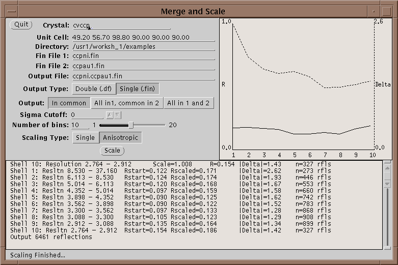
First run your native and heavy atom data sets through Xprepfin to prepare your data; put it in the .fin format. If needed reduce the indices on both sets of files with xprepfin. Run xmerge: specify the native file first and the heavy atom second. Xmerge scales the second file to the first which it leaves unchanged. The program has two file options for the output: another .fin file or a double fin file, .df. The double fin file preserves the Bijvoet differences and the .fin file merges the Bijvoets to a single F. Both files have advantages and disadvantages - however, a .df can be converted to a .fin with xprepfin whereas the opposite is not true. There are two scaling options that can be set, the number of bins of resolution and isotropic or anisotropic scaling. The number of bins should be set such that enough reflections are included in each bin. Too fine a bin will overscale the data and reduce the signal in the differences. A good bin size will give about 100 reflections in the smallest bin. Anisotropic scaling uses 6 scale parameters per bin and so if turned on the number of reflections per bin should be higher - say 500 reflections. After scaling the data, xmerge displays several graphs which can be used to determine the quality of a heavy atom derivative. For more information on how to use these graphs see McRee2.
1.2 Patterson Solutions
XtalView includes a program, Xhercules, designed to automatically solve Patterson maps by using a correlation function computed at every position in the unique volume of the unit cell. The method starts with first 1 atom and then adds a second atom and so forth until the Patterson vectors are fulfilled. To start the procedure a Patterson map is first calculated with Xfft using the differences between either isomorphous pairs or anomalous scattering pairs. The outlier filter should be set to about 100 to filter out ridiculous differences that are usually caused by scatter off the beam stop or the beam stop being slightly different between the two crystals. This map is then contoured with xcontur and left open for later comparison with the output of the automated heavy atom solution procedure. Xhercules works in both the anomalous and isomorphous cases: simply use the appropriate .fin file with Bijvoet pairs in the anomalous case or merged heavy-atom data in the isomorphous case. If you made .df file when using xmerge to merge the native and derivative data, then use xpatpred with the df(1+2,3+4) option to make a .fin file.
For the first position both the hand and the origin are arbitrary so that for an orthorhombic crystal only the volume 0-1/4, 0-1/4, 0-1/4 need be searched. Start xhercules and enter in this volume. Leave all the file fields blank, except for the fin file, which will have the name of your scaled and merged derivative difference data. To verify sites found in xhercules, use xpatpred to see if the predicted vectors for that site agree with the Patterson map. This is done by starting xpatpred and entering the solution. Then use the predict button to write the expected vectors to a file. Then load this file into xcontur as a labels file and overlay the Patterson map. The expected vectors fill the unit cell from 0-1 and thus the bounds of the Patterson must be in this range.
Having decided on a first site, you save this into a solution file with xpatpred and then give xhercules this file as input. This time, when xhercules is run, it will keep the site(s) in the solution file fixed and search for a second site. Having fixed one site is equivalent to making an origin choice, and the unique volume thus increases in an orthorhombic space group to 0-.5, 0-.5, 0-.5. Fixing two sites fixes the hand, and thus one needs to search the entire asymmetric unit for a third site or 0-1, 0-.5, 0-.5 in an orthorhombic case.
To see if a site is correct, it is important to compare the predicted vectors with the actual ones in the Patterson map. For this use xpatpred. Put up the Patterson map with xcontur and also start xpatpred. Enter the heavy atom site into xpatpred by typing in its coordinates from xhercules and selecting Insert. Enter a filename for the Predictions File: - I usually use "pred". Now select the Predict button which writes a labels file for xcontur. In xcontur, select the Files… button, enter "pred" in the Labels: field, and press Load Labels. The file will be loaded as labels filling the volume 0-1,0-1,0-1. You can then look at the Harker sections to see if the self-vectors are there, and, if there is more than one site, look through the Patterson to see if the cross-vectors fall on density. If another program is used to solve for heavy-atom positions or if you figure them by hand, you can still use xpatpred and xcontur to check the positions against the Patterson map.
It often happens that two single sites are evident from the Patterson map, and the problem becomes fixing the relative origin of one site to another. In this case one can use xpatpred to cycle one of the sites through all of the origin choices and simply look in xcontur to see which pair gives the best match to the cross-vectors.
1.4 Bijvoet Pattersons
In XtalView a Bijvoet Patterson is treated exactly as an isomorphous Patterson except that the data are already merged for you by the data reduction program. The .fin file is loaded directly into xfft and a Patterson made using the .fin file input type on the Pattersons Only submenu of the File Type menu. To ensure that the centrics are handled properly, see the section on xprepfin above on preparing Bijvoet pair data.
1.5 Difference Fouriers
Difference Fouriers are implemented with xmergephs which takes as inputs a .fin file and a .phs file. The differences in the .fin file end up being phased with the input .phs file. When making an isomorphous difference Patterson, swap F1 and F2 so that the coefficients to the Fourier map are Fheavy - Fnative. Otherwise the peaks will be negative. For a Bijvoet difference Patterson the phase needs to be shifted by 90 degrees, so set this button on as well. The output is another .phs file which is then run through xfft (or xfit) with the map type set to Fo-Fc which in this case is Fheavy-Fnative. The difference map can be displayed in xcontur. To find the peaks, set the slab to be one asymmetric unit thick and adjust the contour level such that only the large peaks show. Clicking on a peak with the mouse then gives the fractional coordinates which can be entered into the heavy atom solution in xpatpred (see above) and then verified against the Patterson map, which is very important!
In a similar manner a mutant difference Fourier can be made by merging with the native phases. First merge the wild-type and mutant data with xmerge, putting the wild-type as the first file. The order of the F’s are then swapped in xmergephs, so that in the resulting difference map the positive density will indicate new atoms in the mutant and the negative will indicate the missing atoms.
1.6 Heavy-Atom refinement
Xheavy uses a very robust refinement algorithm that is based on a correlation search. It gives very accurate positional parameters. The phasing part of xheavy is somewhat dated at this point, although xheavy has been used to solve many structures. In marginal cases other common programs can provide better phases. With good derivatives the phases end up very much the same although the figures-of-merit cannot be directly compared.
The refinement is done by searching for the maximum of the correlation:
where
D is the difference between the native and the derivative and fh is the calculated heavy atom model. The advantage of using the correlation is that the scale factor drops out of the equation. In the early stages of heavy-atom refinement, the scale-factor is unknown as the degree of partiality of the model is uncertain. The disadvantage is that the maximum must be searched for by trying many positions and keeping track of the behavior. Xheavy uses an algorithm for this search that first chooses a grid based on the upper resolution limit and searches a small area. If a better match is found at the edge of this area, a coarser grid is used. If the shift is small, a finer grid is then tried. If there is no movement, a grid in-between is used, and then a smaller grid is used again until changing the grid has no effect. This allows for a large radius of convergence but takes a long time.
The heavy-atom model can be incomplete, and the correct results will still be obtained. For example in a multisite derivative a single site can be refined alone. Refining each site independently allows for more accurate cross-vectors to be calculated when the relative origins of the sites have not been discovered.
The correlation function roughly indicates the quality of the derivative as follows (to be taken with a grain of salt as these numbers are dependent upon resolution, isomorphism and mood). In general, 0.5 - 0.6 can be obtained with wrong sites, 0.6 - 0.68 indicates something good is happening, and 0.68 - 0.77 indicates good solutions that can provide real phases. Above 0.77 indicates an excellent solution and isomorphism.
Although one may use another program to calculate the final phases, xheavy is very useful for calculating difference Fouriers for cross-phasing other derivatives. A phase file for the SIR or SAS phases can be used with xmergephs to produce a difference Fourier with another merged heavy atom data set.
1.7 Model Building

Xfit is used for model building. Several models and maps can be viewed simultaneously and the usual fitting operations of moving the model to fit the density can be done. I will concentrate here on less common features for fitting programs. The fitting model was inspired by GRIP-75, a University of North Carolina project.
The Mouse. The main input device is the mouse. Since a mouse has only three buttons on UNIX systems, some compromises had to be made. The leftmost button controls the rotation about the center of the screen. The rightmost button brings up a menu of commonly used options. This menu overcomes the back and forth motion of other systems that is needed to select options from a menu. Since there are only three buttons, the middle-mouse button is made to do multiple duty. The right-mouse menu is used to change the middle-mouse function and the cursor changes to give feedback to the user as to what mode is current. The middle-mouse button defaults to dragging the screen center. In early tests it was found that a trackball model of mouse motion was confusing as the user could never be sure exactly which way the model would move - a serious problem in a fitting program. This left us with a need to implement a z-rotation about the center of the screen. To do this Xfit uses the top inch or so of the screen for z operations. Again, the cursor changes to let the user know he is in this region.
Maps and Phases. Xfit has a built-in Fast Fourier Transform capable of going in both directions from phases to maps and from models to phases. This allows a lot of flexibility in the use of the program. For instance the resolution of the map can be changed at any time and the type of map can be changed. To encourage the user to use phase files instead of maps, they are treated in the same way in the program. Besides experimental phases such as MAD and MIR, crystallographic phases are derived from the model. Xfit can calculate these phases if given a reflection list. The reflection list is prepared with xprepfin (as a fake phase file - perhaps better called an empty phase file). This allows updating the phases at any time during the fitting. A partial structure factor calculator also allows making omit maps on the fly.
To use the spline-based maps, set Splines: to quadratic or cubic in the FFT window. The Use Grid: option in the Contour window can then be set to Orthogonal, allowing contour grid spacing to be any desired value in Ångstroms, independent of the FFT grid. We use the spectral spline approximation described in [3]. When the phases are FFT’d, the resulting density is modified by a weighting function so that each element in the density array contains information about density throughout local space. Two versions of the weighting function were tried: one assuming a discrete and a continuous FFT. Although the continuous version had lower mean deviation from the true density value, the discrete version was chosen because it provides a much closer approximation at the FFT grid points themselves.
Placing Ligands and Fragments: A Large Translation Search button is available in the Refine window. This will translate the user’s current fragment to anywhere in the visible contoured density, by superimposing the fragment’s center of mass on the center of the density after subtracting the density of the atoms not in the fragment. Because this center is only an approximation of the desired position, the program follows the large translation search with a standard translation search, which does a brute-force search of nearby positions for the best density correlation.
Starting a New Model de novo. To start a new model, click the model number on the main window to an empty position. Then open the Model window and select the first residue type as a MRK. (If there is no list under the Type menu button, then you need to set up the environment variable $XFITDICT so that the dictionary is found.) Enter in a number for the residue name. If you are not sure what it should be, just set it to something like 100. Turn on the Autonumber function. You are ready to start adding residues. The new residue will be placed at the center of the screen so make sure that the CA position of the first residue is centered on the cross. Now select New Model from the Insert menu button. At this point you can continue inserting more residues by centering their density and using Insert After or Insert Before (the autonumber will add or subtract in naming the residue), or you can use the new autofit functions as described below.
Fixing Main Chain. One of the trickiest parts of fitting is getting the main chain peptide planes correct with good phi-psi’s. In xfit the strategy is to use the positions of the CA and CB atoms to define the main-chain geometry rather than trying to move the peptide plane itself. Five pentamer poly-ala fragments are then fit over the part to be fixed and the geometry of the main-chain is replaced with the new geometry. The functions for this are on the Model window under the Insert menu. The Pentamer menu is a pull-right menu.
2 Interfacing to other programs
This section gives specific information for interfacing to popular software.
Molscript - The xfit script commands rotation and translation can be used to set the viewpoint in molscript. The translation is the inverse of molscript’s, but other than this simple change in sign they can be cut and pasted into a molscript control file.
SHELXL - SHELXPRO has an XtalView command to allow writing sigma-A coefficients into a .phs file. To use these, read in the file as a map file in xfit and make a Fo map. Since SHELXL uses anisotropic B-values and a more accurate structure factor calculation (especially at very high resolution), it is better to use this option than to use the Sfcalc options in xfit. After fitting the SHELXPRO program is used to integrate the changes into the SHELXL .ins file.
DENZO - Xprepfin can prepare input from a .SCA file by choosing Other as the input file type and DENZO I’s from the Other menu. You will note that the F sigmas of Bijvoet differences are fudged. The reason for doing this is so that they will be recomputed properly in the XtalView programs.
CCP4 - The preferred way to use XtalView with CCP4 map files is to use the phase files as input and not map files. This will be faster and save disk space. However, there is a CCP4 map converter available from CCMS that was kindly provided by John Irwin. Send email to ccms-help@sdsc.edu and ask.
PHASES - Xheavy writes an input file for PHASES that will get you most of the way to running PHASES. Look at the menu on the menu button for saving a phase file. In this way you can use xheavy for the heavy atom location and refinement and then switch to PHASES. There is not much difference in the actual phases produced, but PHASES has solvent flattening, and XtalView will not have this until the next release.
XPLOR- Xprepfin can be used to generate an input file for XPLOR Fobs data. If your native data has Bijvoet pairs, be sure to use the Average F1 and F2 option in xprepfin. You can switch the segid with the chain-id in xfit by using the options on the Files… window. Since the chain-id field in a PDB file is 1 character only, the first character in the segid is used. This allows one to get around the fact that XPLOR loses the chain-id.
XPLOR, TNT, PROLSQ and other refinement programs- To make maps, first prepare your native data into an empty phase file with xprepfin and the Fake Phs output option. This creates a file with 0.0 for the phase. Now run xfit, loading the empty phase file and your latest PDB file as refined by XPLOR. The FFT window will pop-up, but don’t hit the Apply button. Instead just set the map type you want (e.g. 2Fo-Fc) and then go to the SfCalc window. In here choose the Calculate All and Scale button. Xfit will calculate Fc and the phase, scale Fo to Fc (to put on an absolute scale) and then FFT your density. If you want to look at an Fo-Fc map as a second map, just reload the phases with the File window and repeat the procedure setting the FFT type to Fo-Fc.
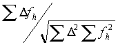
3 Semi-automated fitting
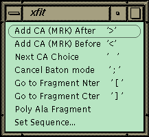
Figure 1 Xfit Auto-fit Menu.
The commands for auto-fitting are on this menu with the keyboard shortcut listed on the right in quotes. Access this on the toolbar.The xfit auto-fit menu is shown in Figure 1. A new object, the fragment, has been added to the program, and the commands in the menu work on the last fragment picked. A fragment is a piece of chain that is not connected to the rest of the structure. The strategy for auto-fitting is to build a CA chain-tracing and then to poly-ala the chain. The sequence is then matched to a point in the chain, and the sequence is automatically built in both directions to the ends of the fragment. The commands allow adding a new residue to either end of the current fragment. The program uses the density and geometry to decide on 6 best positions for the next CA. The CA is placed at the first position and left in refine-while-fit mode with a constraint of 3.5 Å to the last CA (baton mode). The user can step through the 6 positions with the spacebar or use the middle mouse button to position the CA manually. Hitting ">" or "<" proceeds to the next residue directly. If the density is fairly clean, the map can be stepped through very quickly to build a CA chain-trace. The fragment is then poly-ala’ed to form a backbone. The poly-ala command builds overlapping pentamer fragments from the N-terminal end of the fragment to the C-terminal end.
At this point the sequence can be matched to a sequence read in from a file. One CA is picked, and then the corresponding point in the sequence is picked. The program will then replace the side chains for the fragment and fit each side-chain by going through all the conformers and finding the best match to the density.
New commands have been added to the Model window that allow manipulating the fragments and putting them in the correct order. A fragment can be named sequentially, the order reversed, and fragments sorted by sequence number. With the new commands it is no longer necessary to use a text editor in building models.
3 Future Directions
Items which are planned but are not so far along as to be certainties are listed here (this does not include pipe dreams and wild speculations which will be discussed over coffee).
Xheavy - maximum likelihood refinement will be implemented as well as more tightly integrating the heavy-atom finding and picking procedure. B-value refinement will be added as well as heavy-atom groups.
Xfit - Sigma-A maps will be computed directly in the program using the current model and the heavy-atom coefficients. OpenGL support will be added as well as solid-surface maps and ball-and-stick models.
4 Summary and Conclusions
The new autofit commands greatly simplify model building in xfit and result in improved geometry for the initial model. Several new structures have been built at Scripps using these techniques and they have all refined rapidly.
XtalView is distributed by CCMS and is available for SGI, SUN, DEC (OSF) and LINUX. To receive information on downloading XtalView send an email to ccms-request@sdsc.edu with a blank subject and the message ‘get xtalview’. Instructions will be sent by return email. CCMS has a staff of consultants to answer your questions and solve problems at ccms-help@sdsc.edu. Commercial users should contact Mary Donlan, MSI, (619) 546-5532.
References
[1] D.E. McRee, "A visual protein crystallographic software system for X11/XView," J. Mol. Graphics, Vol. 10, pp. 44-46, 1992.
[2] D.E. McRee, Practical Protein Crystallography, Academic Press: San Diego, 1993.
[3] E. Nelsen and L. Ten Eyck, An efficient local analytic representation of electron density maps: the spectral spline approximation. Abstracts of the XVII International Union of Crystallography, MS21.02.05, pg. C-555, 1996.