MAD Phasing with XtalView
With the proper treatment, xheavy can be used to phase MAD experimental data. No modifications are needed to the program and the method used is similar to that used by others to phase MAD data by treating it as a special case Of MIR phasing. The anomalous differences between Bijvoet pairs are treated as native anomalous and the dispersive differences between wavelengths are treated as isomorphous pairs. Care must be taken to treat the member of the dispersive pair with the smaller f' as the native while the other is the derivative.
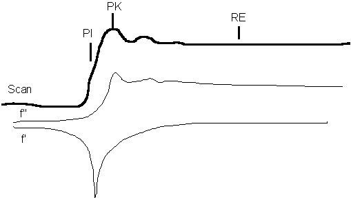
First some nomenclature. MAD experiments are done by measuring 3 or more wavelengths. The 3 wavelengths are identified by an XAS scan at the absorption edge of the anomalous scatterer in the crystal:
PI - point of inflection of the edge, minimum of f'
PK - peak of absorption above the edge in energy, maximum of f''
RE - remote edge above the edge in energy, maximum of f'
Additionally, a 4th wavelength is often measured below the edge. Its contribution to phasing is minimal although it may increase redundancy. It would be handled identically to RE except that it will have no anomalous signal. More useful may be another remote edge above the edge in energy which would have both a dispersive difference and an anomalous signal. Call this wavelength RE2.
The best way to collect the data seems to be to simply collect 3 data sets on a frozen crystal with exactly the same strategy. Make sure you collect enough data to get about 95% completeness on the Bijvoet pairs. Offset the crystal that it rotates about 20º off an axis to up the completeness by avoiding the blind zone overlapping an axis. We monitor the data by integrating it continuously as it comes off the machine to find the point at which the data is complete and to make sure we are getting good R-symms. The quality of the data is the ultimate key to MAD phasing. We have tried strategies to collect the data in blocks and find this unnecesarily complicates data collection, reduction and phasing. Our best results have come from the simplest strategy. R-symms should range from 2-3% for the low resolution data to 10% for the high resolution with an average of about 6% (wihtout merging Bijvoets).
The Bijvoet differences are treated as would any anomalous scatterer. Make the Patterson maps as usual with xfft. The dispersive differences need to be merged with xmerge. Merge the pairs in this order:
PI-PK
PI-RE
PK-RE
The largest signal will be in the PI-RE pair. All 3 wavelengths, PI, PK and RE will have an anomalous signal with the largest signal at PK. If you can't see peaks in the Patterson maps at low resolution - say 5 A, then there probably isn't any need to proceed. However with well measured data this should not be a problem. we have seen sulfur atoms in Bijvoet difference Pattersons.
Solve the Patterson with xhercules if it can't be solved by "hand". You can also use SHELX if the Patterson is complicated. One thing missing from XtalView is the means of making FA coefficients, i.e. combining all the possible pairs together to strengthen the signal. So far we haven't been hindered by this as we have been able to easily solve all of our Pattersons.
In general, if there isn't anything in the Patterson map, then its not worth including this pair in the phasing.
Now you are ready to phase. Start xheavy and use the editor to add each pair. You will have 6 "derivatives": PI_ano, PK_ano, RE_ano, PI-PK, PI-RE and PK-RE. In order to avoid overestimating the figure merit each derivative should be weighted correctly. Weight each derivative at 33%. This way the problem reduces to 1 isomorphous derivative plus one anomalous derivative. If you have an RE2 derivative, lower the weights to 25% since you now have 4 identical solutions. Failure to downweight will hinder the solvent flattening step by not giving any room for improving the phases. All the derivatives share the same sites - call them all PT (the default - in practice the subtle difference between different atom types structure factors are far below your noise levels) and set the B's to 10.0. Refine the derivatives as usual. Start at 5 Angstroms and then raise the resolution limit to whatever limit you feel the signal continues to. Be honest here- adding lots of high resolution but poorly phased data will not help the maps. One problem is what to call the native F. If you have a data set you plan to use as the native for refinement then include this on the master fin file field.
Once refined you can calculate the protein phases. During phasing you get several useful statistics. One is the R-anomalous of the 25% largest Bijvoet differences for the anomalous pairs. This should be 40% or less. 25-30% is ideal. The R-centric can be used for the isomorphous/dispersive pairs. These should be 60% or less. In the 50's is ideal. Another thing to check is the acentric and centric scale factors which should agree within about 20%. The differences in the values of f' and f'' are all automatically scaled by xheavy. The phasing power for the dispersive pairs is usually surprisingly high if you are used to heavy atom derivative phasing. This seems to be because the errors are quite low since the same crystal is used for all measurements. The final figure-of-merit in our cases has been in the 60's. This would seem low for a normal MIR experiment but the equivalent MAD maps are much better.
At this point you MUST try BOTH alternate heavy atom configurations, as called "hands". The correct configuration is ambiguous in the Patterson function and cannot be found a priori. To try the alternate invert each atom around the center - i.e. change the sign on x,y,z to -x,-y,-z. Make both maps and examine them in xcontur. In one you will see clear solvent channels and protein features and the other map will be junk. If you can't see a difference backtrack and check all the steps.
At this point its worth looking for minor sites (unless the maps are so good you don't need to). What minor sites you say? Why the sulfurs of course. The sulfurs in the protein will have no dispersive signal as they have no absorption edge in the range useful for MAD. However, they do have a small but significant anomalous signal. By making a Bijvoet difference Fourier map using xmergephs (check both iswap and add 90 degree check boxes), the PK.fin dataset and the current protein phases you can look for peaks by making a 5-4 Angstrom Fo-Fc map in xfft and then using xcontur and add these to the anomalous solutions. Then recalculate the phases. This Bijvoet difference Fourier map is also very useful for finding the sulfurs in cysteines and methionines to verify your sequence assignment and finding sequence markers. We have been using this technique with great success for a number of years in all our structure solutions. Even though the resolution at which the sulfurs can be seen is usually quite low, 5-4 Angstroms, this is more than sufficient for locating the sulfur containing side-chains for sequencing purposes.
One note. the site of the scatterers will be the worst spot in the map. The reason for this is quite technical but has to do with all the errors piling up at the spot where the heavy atom is located since it effectively defines the origin of the phasing. They usually come back with solvent flattening and in the first map after refinement.
Now you are ready to fit the maps! E-mail me with difficulties and/or questions. We have solved three proteins in the last year with MAD and XtalView. Our record is a molecule with one Fe in 53,000 kDa - which I believe is probably a world record - the theoretical signal is only 1.4%. We were also able to find the sulfurs in the Bijvoet differnce Fouriers. We have also solved another heme cytochrome as well as a Cu-Cu protein.