Retrieving and Processing BT-1 Files

 

Retrieving files

  

Figure 20: The initial window from rem_fetch.

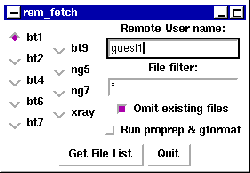
After data has been collected, it can be transferred using the UNIX command, rem_fetch. When this command is invoked, a graphic user interface (GUI) appears, as seen in Fig. 20. For the ``Remote User Name'' enter the directory used to collect data, for example, guest1 for [BT1.GUEST1] or sam.nano for [BT1.SAM.NANO]. Press the ``Get File List'' button to see a list of files displayed. By default, all files in the appropriate CNBS directory are then displayed (as seen in Fig. 21), except that files previously transferred into your current directory are not included. This behavior can be changed by deselecting the ``Omit existing files'' checkbutton, which causes all files to be displayed. It is also possible to select the files that will be listed using the ``File filter.'' For example, use of *ac* for a file filter restricts the file list to files containing the string ``ac''.

  

Figure 21: A list of files displayed in rem_fetch.

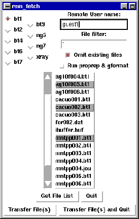
After the ``Get File List'' button is pressed, the window is modified to include the file list, as seen in Fig. 21. At this point it is possible to modify any of the previously described fields and then press the ``Get File List'' button to obtain an updated list.

Multiple files are selected by clicking on them while holding the shift key down, or groups of files can be selected by using control while clicking on them. Once a set of files has been selected, pressing the ``Transfer File(s)'' or the ``Transfer File(s) and Quit'' button causes the files to be transferred to the local computer. If the ``Run proprep & gformat'' checkbutton is selected, each file is individually processed by the proprep and gformat programs (see below) as the files are transferred.

Processing files

Program proprep is used to convert BT-1 data files to an intermediate format where data are separated by detector number. The gformat program may then used to scale, interpolate, and combine the data to appear as if it were collected using a single detector.

proprep

Program proprep is used to convert .bt1 files into .raw files used by a number of programs, such as REFINE and are used as an intermediate for conversion to GSAS format. It can be used to add multiple runs, but this is better done in program gformat, if files for GSAS are to be produced.

The program can be used by typing:

       proprep file

or

       proprep file.bt1

Either command causes file file.bt1 to be read and a new file, file.raw, to be created. Several (up to 50) files can be processed at one time:

       proprep file1 file2 file3

or even,

       proprep abc*.bt1

where the .bt1 extension is assumed if not specified. The program will produce an error message and fail if the .raw file exists.

It is important to look carefully at your data before execution of proprep. For instance, you may wish to exclude data below 5 degrees in detector 1, 10 degrees in detector 2, and 15 degrees in detector 3 using the option -cx.x (see below), as the background levels in these regions is often anomalously large. The default is to exclude data below 3.0, 8.0, and 13.0 degrees, respectively for detectors 1, 2 and 3, which would affect only data taken with the Ge(311) monochromator under standard data collection conditions.

A number of options can be supplied to proprep:

       proprep [-s] [-k] [-1] [-cx.x] [-dx,y] [-p] file1 [file2] ...

or proprep can be used as a filter:

       proprep -f [-k] [-1] [-cx.x] [-dx,y] < file.bt1 > file.raw

The full list of options accepted by proprep follows. Options can be combined together where appropriate.

-s

sum all specified files into a single file. The file will be named using the first input file. Use of gformat rather than proprep for this purpose is recommended because gformat checks that the files are in statistical agreement.

-k

keep all data from detectors 1, 2 and 3.

-1

keep all data from detector 1, but discard data below a threshold from detectors 2 and detector 3 (used to preserve very low angle peaks).

-cx.x

Sets the threshold for cutting low angle data from detectors 1, 2 and 3 (unless -k or -1 is used). The default threshold is 3.0 meaning that data below 3.0, 8.0 and 13.0 degrees are cut from detectors 1, 2 and 3, respectively. This means that by default, data is only cut from Ge(311) scans.

-dn

drop data from detector n, or if more than one number is used, for example, if ``-d1,3,5'' is used, data from banks 1, 3 and 5 will be dropped.

-p

pipe output to stout rather than create an output file.

-f

run as a filter: read from stdin and write output to stdout.

gformat

Program gformat is used to convert .raw files into pseudo-single-detector .gsas files that are used by GSAS and a few other programs. The zero corrections and scale factors found in the .bt1 file header (and written in the .raw file) are applied to the data. The program can be used to add together runs of different lengths, but the first file specified should start at the lowest angle. When points are averaged together, a statistical check is applied to see how well the points agree. Warnings about points that differ by more than $4\sigma$ are appended to the end of a file named stat.check. When warnings are generated, a message is displayed on the user's terminal.

In the simplest form, program gformat is used by typing,

       gformat abc.raw

to process abc.raw into abc.gsas. Note that the .raw extension is assumed if not specified for input files, so that the command

       gformat abc

is equivalent to the previous command.

Up to 50 files can be specified on the command line. Each will be processed individually (unless -s is present, which causes the contents of the files to be averaged, see below). To process a series beginning with the letters ``abc'' you can use the commands

       gformat abc*.raw

Background corrections are applied to each detector bank to give the best agreement for overlapping data. This correction can be omitted using the -o option. The program will not overwrite an existing .gsas file unless -c is specified.

When a zero correction is applied to each detector bank, data points will no longer ``line up'' with the data points in the output file. Thus, gformat will interpolate the intensity for each point when it bins. This creates some correlation between adjacent points, which is not strictly appropriate for correct least-squares statistics. If -m is used the points are placed into the closest bin without interpolation. This introduces a bit more scatter into the data, but is statistically more valid. The -m option causes your output step size to be double that of your input, which reduces the scatter that is introduced, so if you are going to use -m, you should probably collect data with a smaller step size 0.02 or 0.025 degrees).

The data for all detector banks is included in the .gsas file, unless the -L option is used (see below). A .inst file is created with the same file name as every .gsas output file. This contains the wavelength and other sundry information.

The .gsas and .inst files created by gformat can be e-mailed, ftp'ed etc. However, before using the files in GSAS, they need to be converted to direct access. This is done automatically for use with UNIX versions of GSAS by gformat. The direct access data files are named with all capital letters. When using e-mail or for non-UNIX versions of GSAS, transfer the lower-case named files.

A number of options can be supplied to gformat:

       gformat [-s] [-c] [-o] [-m] [-Lxx] [-a] file1 [file2] ...

or gformat can be used as a filter:

       gformat -f [-Lxx] [-o] [-m] [-a] < file.raw > file.gsas

The full list of options accepted by gformat follows. Options can be combined together as appropriate.

-s

average all specified files into a single file. The file will be named using the first input file.

-Lxx

discard the data from detector number xx and subsequent detectors.

-c

overwrite existing .gsas file(s) rather than stop.

-m

move points to closest bin rather than interpolate.

-o

don't apply a detector-by-detector background spline correction.

-a

apply an absorption correction using the coefficients from file abs.corr

-f

run as a filter: read from stdin and write output to stdout.

The -g option requires an absorption correction input file, abs.corr, which consists of a free-format file containing a one-line title followed by the number of Chebyshev terms (up to 30) and the Chebyshev polynomial coefficients. The polynomial is evaluated for

$$x = 2\theta/90. - 1$$

and the intensity and standard uncertainty (esd) are multiplied by the result. Typically this polynomial is fitted to A* values from the International Tables.

Plotting BT-1 files

 The cmpr program can be used for plotting data in a variety of formats. Figure 22 shows the dialog box used for reading data. Note that pseudo-1D data is processed by the gformat program while multi-detector data does not combine the individual detectors (but does apply the zero offset and efficiency corrections). To read a file, select the format, select the file to be read and click on ``Read Selected File.'' It is also possible to read a file by double-clicking on it.

  

Figure 22: The cmpr read dialog

Files can also be read by starting cmpr with a command option:

      cmpr -readopt file1 file2 -readopt file3

The following read-options are available:

-1d

The following files are to be converted to pseudo-1d data

-md

The following files are to be read as muilti-detector data

-gsas

The following files are to be read as GSAS data

-x7a

The following files are to be read in BNL X7A format

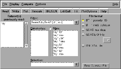
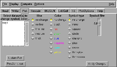
After data has been read, it can be plotted using the dialog box in Figure 23. Multiple files can be selected for plotting using shift plus the left mouse button and then using the ``Update Plot'' button (or double-clicking). It is also possible to change the way one or more files are displayed by selecting the files then selecting options for the Line, Color, or Symbol and then pressing ``Apply Changes.''

  

Figure 23: The cmpr plot dialog

Note that when a file is plotted, it is possible to ``zoom-in'' using the left mouse button to click on two corners of the new region. The right mouse button zooms out and the middle mouse button opens a window for manual scaling.

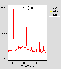
The HKLGEN and EditCell dialog boxes (see Figure 24) are used to generate the allowed reflection positions for a given set of unit cell parameters and optionally using space group extinctions. In EditCell, these reflection positions can be superimposed as vertical lines on one or more sets of data. The cell parameters can be changed and the reflection positions will shift as the lattice constants change. Also, extinct reflections can be highlighted. To see the indices for a reflection, shift-click on the line.

  

Figure 24: Generating and displaying reflection positions in cmpr

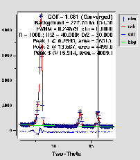
The cmpr program can also be used for peak fitting, as shown in Figure 25. The program uses the GPLSFT program, as written by David Cox and Larry Finger, to do the actual fitting.

To fit one or more peaks, first select the dataset to fit, then zoom-in to the region to fit using the left-mouse button and press ``Set range from graph'' (or manually enter the 2-theta range). Peaks may be entered or modified by clicking on the appropriate ``Set'' button and then by clicking on the appropriate location on the graph. The ``Use'' checkbuttons select if a peak is included in the fit. The remaining checkbuttons determine the variables that are refined when the ``Run GPLSFT'' button is pressed.

  

Figure 25: Peak fitting in cmpr

The cmpr program has other options. For example, the Rescale dialog can be used to multiply or add a constant to a dataset's x-axis or y-axis. It can also be used to change the units for plotting a dataset. For example, intensities can be shown on a logarithmic scale or 2-theta can be converted to 2-theta at different wavelength, or d-spaces or Q. PlotOptions controls how PostScript output is treated. A command for plotting the output, or the name to be used for saving output, can be specified here.

Writing files to floppy disk

Files can be transferred to a DOS format floppy disk quite simply.

1.

Create a UNIX window on the console computer by pressing the ``BT1'' button on the button bar to the lower right of the screen.

2.

Insert a formatted 3.5'' floppy disk in the approporiate slot.

3.

Type the following command:

       mount -v /a

the computer will respond:

       /dev/fd0 on /a type vfat (rw,noexec,nosuid,nodev)

or will report an error.

4.

Transfer files to the floppy. This can be done in a single step, by transferring files directly, or by moving files from another computer, such as rrdjazz. One should not run gformat on directly on a floppy, however, because DOS disks cannot contain two files having the same name, but differing in the use of capitalization (e.g. MYRUN001.GSAS and myrun001.gsas).

(a)

Transfer files directly to floppy:

        (cd /a/; rem_fetch)

(b)

Copy files from jazz. The following command copies all files names beginning with a lower case letter, to the floppy from subdirectory sunysb in account guestbt1 on jazz.

        scp "guestbt1@jazz:sunysb/[a-z]*" /a/

to include subdirectories use scp -r ... in the above command.

5.

Check the contents of the floppy

        ls /a/

6.

Unmount the floppy. (This is important!)

        umount -v /a

The computer will respond

        /dev/fd0 umounted

If the computer responds

        umount: /a: device is busy

you have a process running in the /a/ directory. Type

        cd

in all UNIX windows or if need be log out or all windows (other than the ICP process) on the console until you can run the umount command without an error.

7.

Remove the floppy.